
What Actually Moves Stock Prices?
A practitioner's framework for the 5 forces that determine equity prices, when each one matters, and how to monitor them in real time.

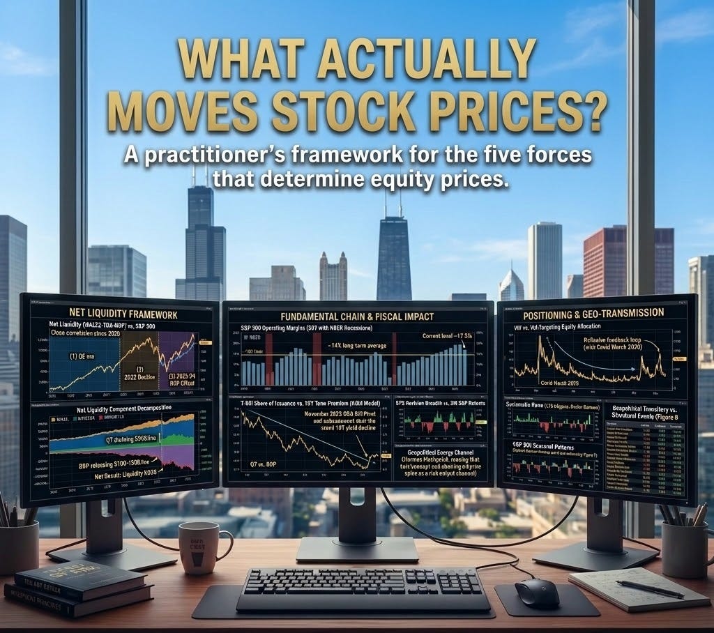
What Actually Moves Stock Prices?
A practitioner’s framework for the 5 forces that determine equity prices, when each one matters, and how to monitor them in real time.
I’ve spent years building and refining the analytical framework I use to assess equity markets. It’s not a model that spits out a price target. It’s a way of thinking about which forces are driving prices at any given moment, how those forces interact, and when the market’s behavior is likely to shift.
Most investors focus on one thing: either they’re watching the Fed, or they’re watching earnings, or they’re watching the news. The problem with single variable thinking is that equity prices are the output of a multi channel system. 5 distinct forces feed into the S&P 500 at all times. Some of them are mechanical and measurable. Others are psychological and harder to pin down. They can reinforce each other, cancel each other out, or occasionally all push in the same direction at once (which is when the biggest moves happen).
I’m going to walk through my framework for how I think about all 5 of these forces, how they transmit into prices, and which ones dominate at different time horizons. At the end, I’ll share the specific data sources and monitoring workflow I use to track them in real time.
This is the kind of post I wish someone had handed me ten years ago.
Why does this framework matter?
Here’s the short answer: equity prices are just two variables multiplied together.
S&P 500 Price = Earnings Per Share (EPS) x Price-to-Earnings Multiple (P/E)
That’s it. Every dollar of market movement can be decomposed into one of two buckets: either earnings changed, or the multiple changed. The 2023 rally, for example, was roughly 75% multiple expansion and only about 25% earnings growth. If you were only watching earnings, you would have missed three quarters of the move.
The 5 forces I’m about to describe ultimately flow into one or both of those two variables. The fundamental forces (earnings, fiscal policy) primarily affect EPS. The financial plumbing forces (liquidity, positioning) primarily affect the multiple. Geopolitics can hit both. Knowing which channel is driving returns at any moment is the difference between understanding the market and being confused by it.
The diagram below is the master map (download for a better quality image). All 5 factors on the left, their transmission channels through the middle, converging on two variables (EPS and P/E multiple) on the right, which multiply to produce the S&P 500 price.
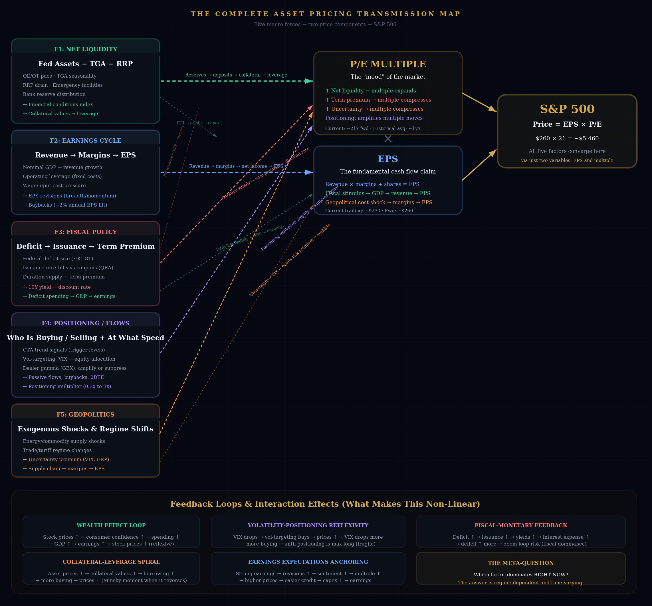
Let me walk through each one.
Force 1: Net Liquidity and Financial Conditions
This is the force I believe is most underappreciated by the average investor, and it’s the one I’ve spent the most time studying. I’m not alone in this view, but it’s still far from consensus.
The Federal Reserve’s balance sheet creates the base money that powers the financial system. But the Fed’s total assets alone don’t tell you how much liquidity is actually circulating. Two massive pools of money sit on the Fed’s balance sheet without being available to the private sector: the Treasury General Account (the government’s checking account) and the Reverse Repo Facility (where money market funds park cash overnight).
The formula is simple:
Net Liquidity = Fed Total Assets - TGA - RRP
This captures the majority of the bank reserves that are actually available to the financial system. When reserves are abundant, funding is easy, collateral values rise, leverage expands, and investors take more risk. When reserves are scarce, the entire transmission chain works in reverse.
The diagram below traces the full transmission stack from reserve balances at the Fed down to the P/E multiple on the S&P 500. Each layer represents a measurable intermediary variable.
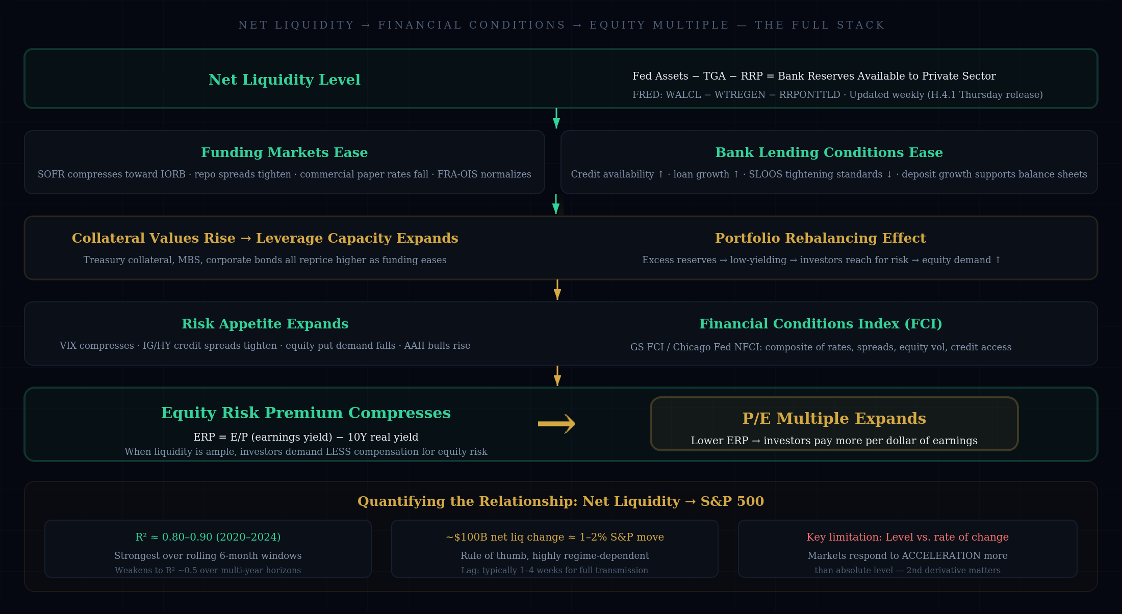
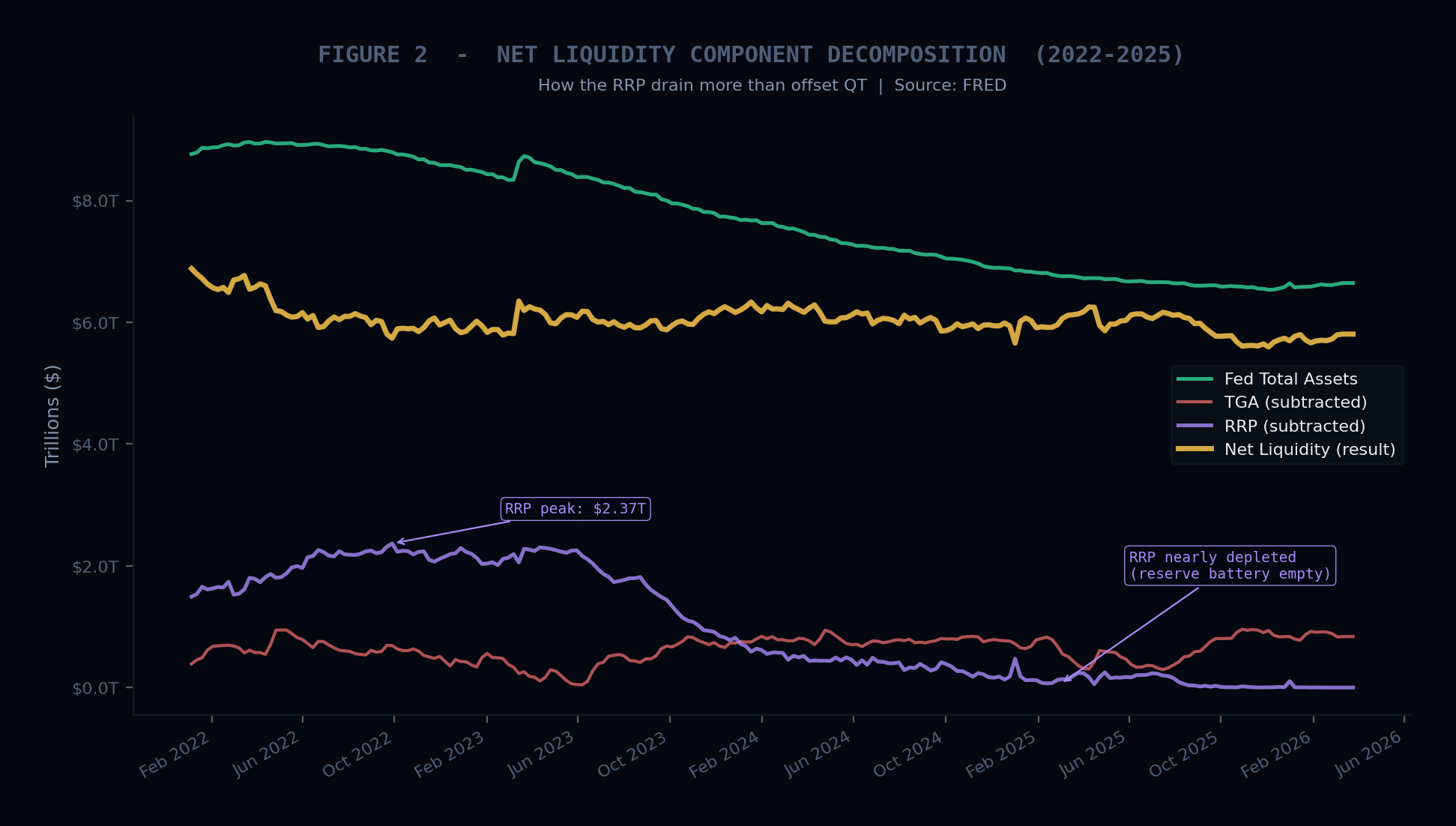
The correlation between net liquidity and the S&P 500 has been striking since 2020, and even going back to 2008 when the Fed entered the ample reserves framework. The R-squared between these two series over rolling 6 month windows has been approximately 0.80 to 0.90.
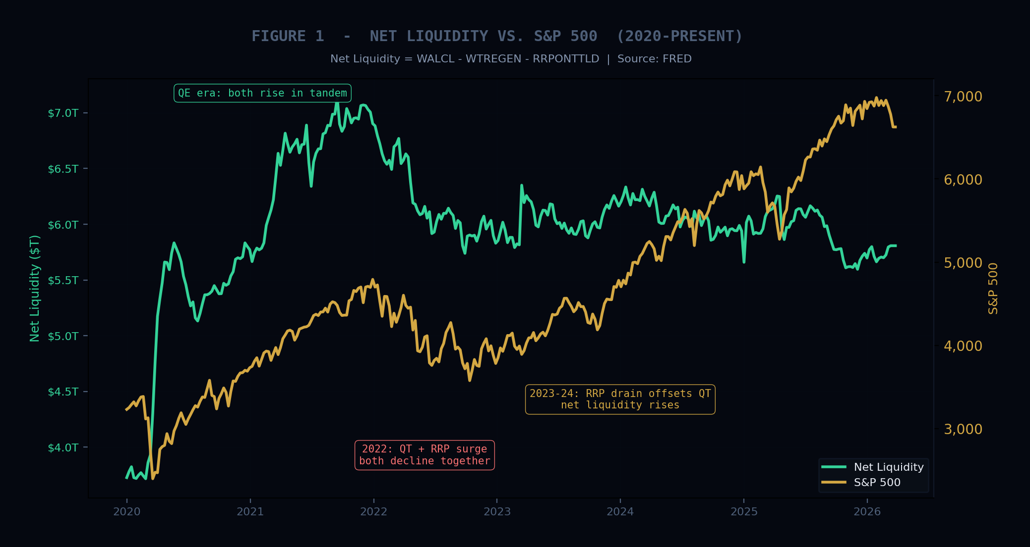
The critical insight about the 2023 and 2024 rally is that the Fed was running quantitative tightening (draining roughly $60 to $95 billion per month from the balance sheet), but the RRP was simultaneously draining at an even faster pace as money market funds rotated into T-bills. The RRP went from $2.55 trillion at its peak in December 2022 to roughly $100 billion by early 2025. That released over $2.4 trillion back into the financial system, more than offsetting the QT drain. Net liquidity actually increased slightly during a period of supposed monetary tightening.
Most analysts watching only the QT headline missed the larger, offsetting RRP flow. The formula captured what they missed.
My conviction level on this factor: high for horizons of 1 to 6 months. Over that window, net liquidity changes have explained an outsized amount of S&P 500 variance. But the correlation weakens considerably over longer horizons, which brings us to the second force.
Force 2: Earnings, Margins, and the Fundamental Chain
Over the long run, stock prices follow earnings. Full stop. Every serious study of long term equity returns confirms this. The multiple gyrates wildly over months and quarters, but over years and decades, it tends to mean revert. Earnings compound. That’s what drives long term wealth creation.
The earnings transmission chain runs from macroeconomic conditions down to the share price. The diagram below shows every layer of this chain (download for a higher quality version of the diagram).
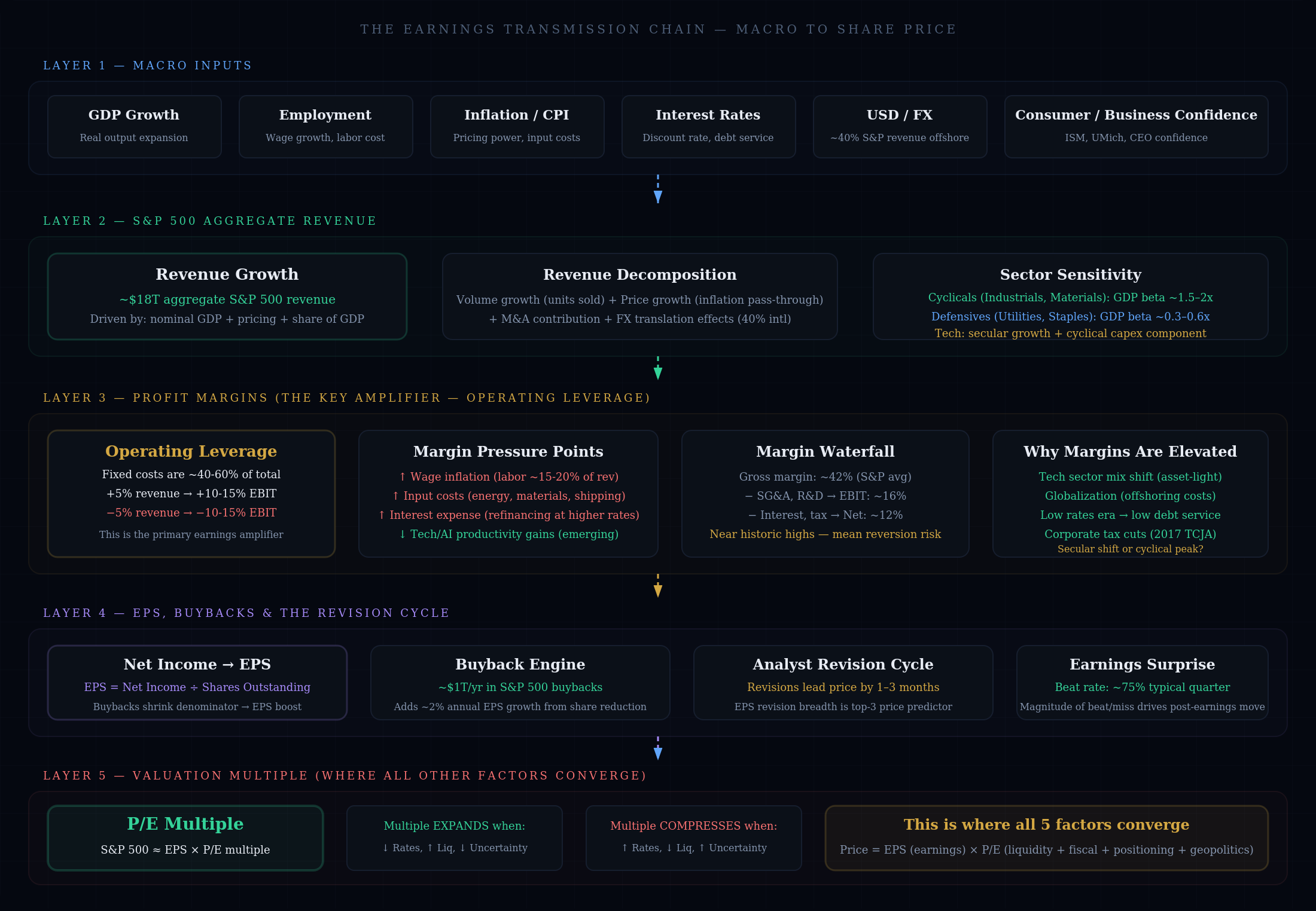
Macro inputs (GDP growth, employment, inflation, interest rates, the dollar) flow into aggregate revenue. Revenue then passes through the operating leverage filter, which is the key amplifier. Because roughly 40 to 60 percent of corporate costs are fixed, a 5% change in revenue can produce a 10 to 15% change in operating income. This is why earnings are more volatile than GDP. This is why recessions produce earnings declines that feel disproportionate to the economic slowdown.
After margins, we get to EPS, which also benefits from the buyback engine. S&P 500 companies are buying back roughly $1 trillion per year in their own stock, shrinking the share count and adding approximately 2% per year to EPS growth even if net income is flat. This is a structural tailwind that most individual investors don’t fully appreciate.
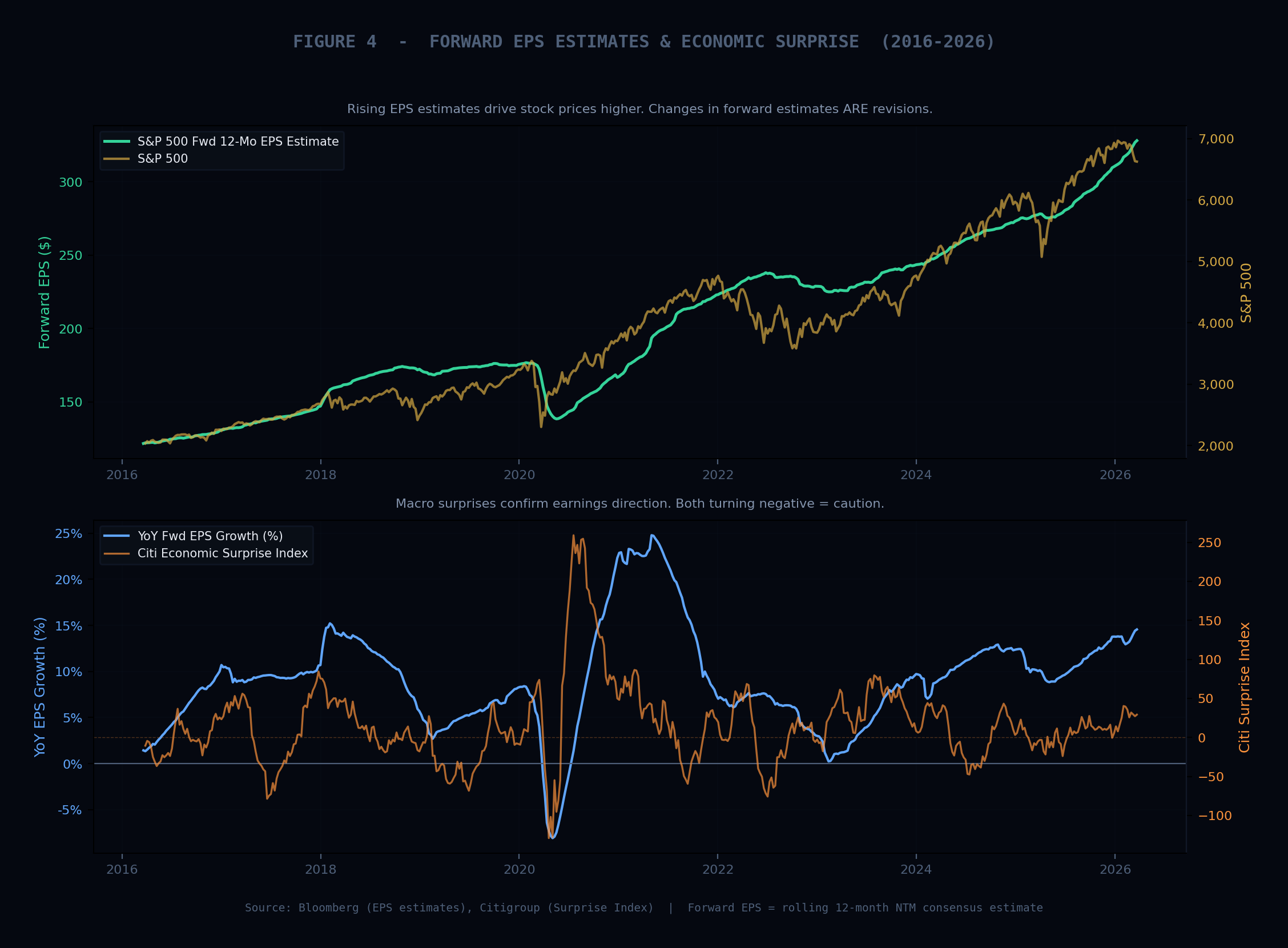
The final and most actionable part of the earnings chain is the revision cycle and growth rate in forward EPS estimates. Analyst EPS revisions (the breadth and direction of estimate changes) tend to lead stock prices by 1 to 3 months. When the percentage of analysts revising estimates upward exceeds those revising downward, the market tends to follow. As positive revisions increase it leads to a rise in forward EPS growth and EPS estimates. This is a direct positive influence on the EPS variable in our formula:
S&P 500 Price = Earnings Per Share (EPS) x Price-to-Earnings Multiple (P/E)
EPS revision breadth and the YoY growth rate of forward EPS estimates are two of my favorite leading indicators for equity direction.
My conviction level on this factor: highest for horizons of 1 to 5 years. Over those timeframes, earnings growth becomes the dominant driver as the multiple mean reverts. For horizons beyond ten years, your starting valuation (Shiller CAPE, for example) becomes the most reliable predictor, because both the earnings cycle and the multiple cycle mean revert over very long periods.
Force 3: Fiscal Policy and Treasury Issuance Strategy
I believe this is the most underappreciated force among all 5, even among professional investors. Most investors think about fiscal policy as “stimulus or no stimulus.” That’s the surface level. The real action is in how the deficit is financed.
The federal deficit is currently running around $1.8 trillion annually, roughly 6.5% of GDP. That’s historically extreme for a non recessionary period. But the size of the deficit alone doesn’t tell you the equity market impact. What matters for asset prices is the composition of Treasury issuance: specifically, the split between T-bills (1 year or shorter) and coupon securities (2 to 30 years).
The mechanism is important to understand:
When Treasury issues T-bills, money market funds tend to buy them using cash that was previously parked at the Fed’s RRP facility. This effectively moves cash from the RRP (trapped, not circulating) into the TGA, and then when Treasury spends, that cash flows into the banking system as reserves. Net effect: more bills equals more reserves equals looser financial conditions equals higher equity multiples.
When Treasury issues coupons (longer dated bonds), those are purchased by banks, pensions, and hedge funds using existing reserves. The duration supply increases, which pushes the term premium higher, which raises the 10 year yield, which raises the discount rate applied to future cash flows, which compresses the P/E multiple.
The diagram below traces this entire chain.
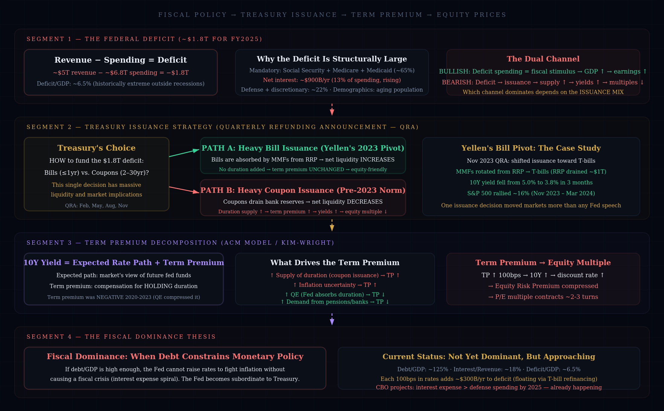
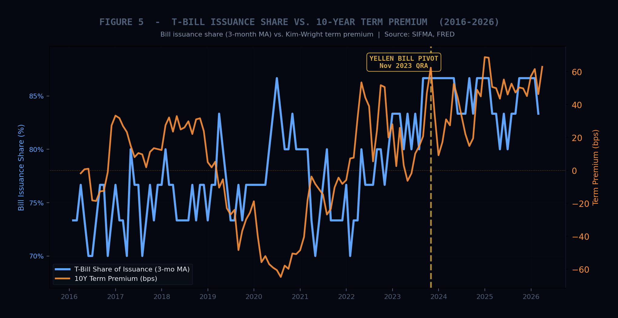
This is exactly what happened in late 2023. Treasury Secretary Yellen shifted the issuance mix heavily toward T-bills in the November Quarterly Refunding Announcement. Money market funds rotated from the RRP into bills, the RRP drained rapidly, reserves reentered the banking system, the 10 year yield dropped from 5.0% to 3.8% in about three months, and the S&P 500 rallied 16%.
One issuance decision. No rate cuts. No QE. Just the composition of how the deficit was financed. That’s the power of this channel.
The quarterly refunding announcement (released in February, May, August, and November) is now one of the most important scheduled events for equity markets. In my humble opinion, it deserves more attention than most FOMC meetings.
The fiscal dominance question also looms. With debt to GDP at roughly 125% and net interest expense now exceeding $900 billion annually (larger than the defense budget), each 100 basis point increase in rates adds roughly $300 billion per year to the deficit. This creates a feedback loop: higher rates increase the deficit, which increases issuance, which can push rates higher. Whether this loop becomes destabilizing is one of the most important open questions in macro.
My conviction level: high, and I think the market consistently underprices this factor. The QRA is a 4x per year event with massive equity implications that most retail investors have never heard of.
Force 4: Positioning, Flows, and Market Microstructure
If the first 3 forces determine where the market “should” go based on fundamentals and plumbing, this fourth force determines how it actually gets there. Positioning is the amplifier (or dampener) of every other signal.
The same earnings beat can produce a 2% rally or a 0.5% shrug depending on how the market is positioned. I think of positioning as a multiplier that ranges from about 0.3x (fully invested, positive gamma, suppressed vol) to about 3x (underweight, negative gamma, light positioning). The fundamental signal is constant. The positioning multiplier changes the realized move.
The diagram below maps the entire systematic flow ecosystem.
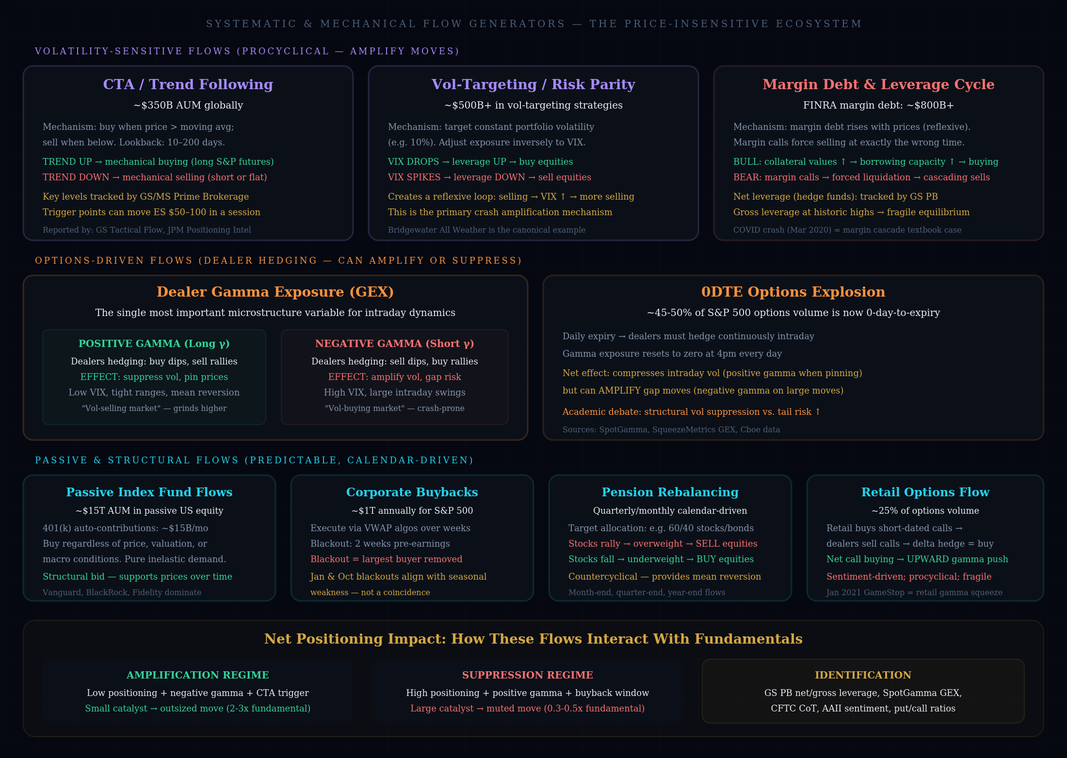
CTA (managed futures) trend following funds represent roughly $350 billion in assets that buy or sell based entirely on price trends relative to moving averages. When the S&P breaks above key trend levels, CTAs mechanically buy futures. When it breaks below, they sell. When a CTA trigger level gets hit, the resulting mechanical flow can move the S&P 50 to 100 points in a single session.
Volatility targeting strategies (including risk parity) manage roughly $500 billion and adjust their equity allocation inversely to volatility. When VIX drops, they increase exposure (buy equities). When VIX spikes, they reduce exposure (sell equities). This creates a reflexive loop: selling pushes VIX higher, which triggers more selling. This is the primary crash amplification mechanism in modern markets.
Dealer gamma exposure is arguably the single most important microstructure variable for understanding intraday dynamics. When dealers are long gamma, they hedge by buying dips and selling rallies, which suppresses volatility. When dealers are short gamma, they amplify moves. The explosion of 0DTE options (now roughly 45 to 50% of all S&P 500 options volume) has made gamma dynamics even more important.
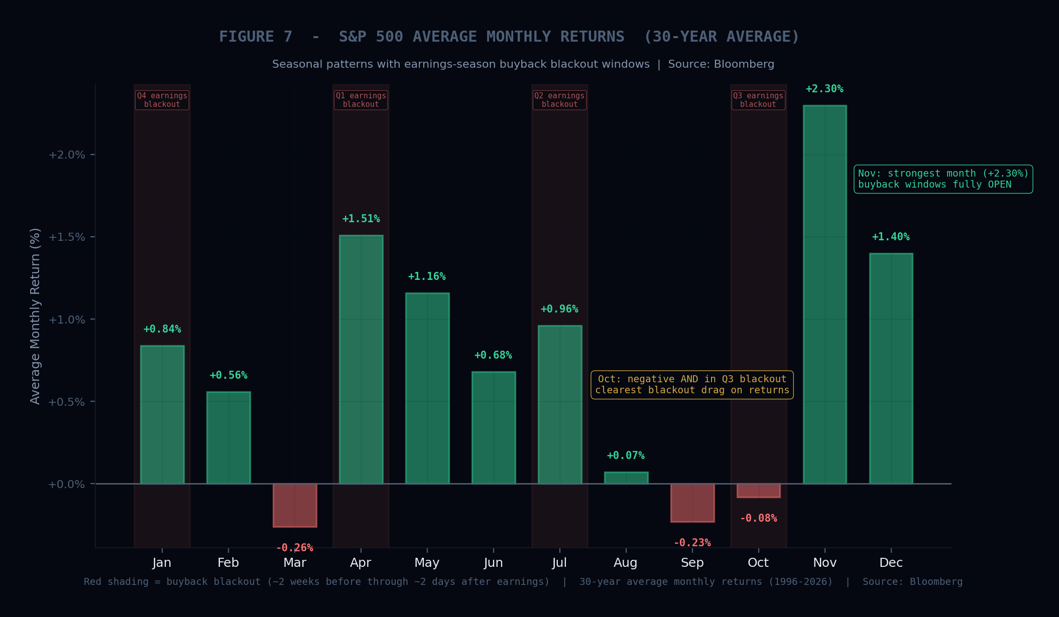
Passive index fund flows provide a structural, price insensitive bid. Automatic 401(k) contributions push roughly $15 billion per month into equity index funds regardless of valuation. Corporate buybacks add another $80 billion or so per month on average, though these come with blackout windows around earnings that remove the largest buyer for roughly two weeks each quarter.
The October 2023 to March 2024 rally is a textbook example. Earnings growth was moderate (5 to 7%), but positioning was extremely light, CTAs hit trigger levels and flipped long, 0DTE gamma pinning suppressed volatility which triggered vol targeting buying, and buyback windows opened post earnings. The positioning setup created a mechanical buying machine that drove the market up over 20% in 5 months.
My conviction level: moderate but increasing. I believe positioning is becoming more important over time as systematic strategies grow as a share of total market volume.
Force 5: Geopolitics, Policy Shocks, and Regime Shifts
This is the wild card. Unlike the other four forces, geopolitical shocks are discontinuous and difficult to model in advance. But their transmission channels are identifiable, and having a framework for how to think about them is far better than reacting emotionally when the headlines hit.
Geopolitical events transmit into equity prices through 5 channels, mapped in the diagram below.
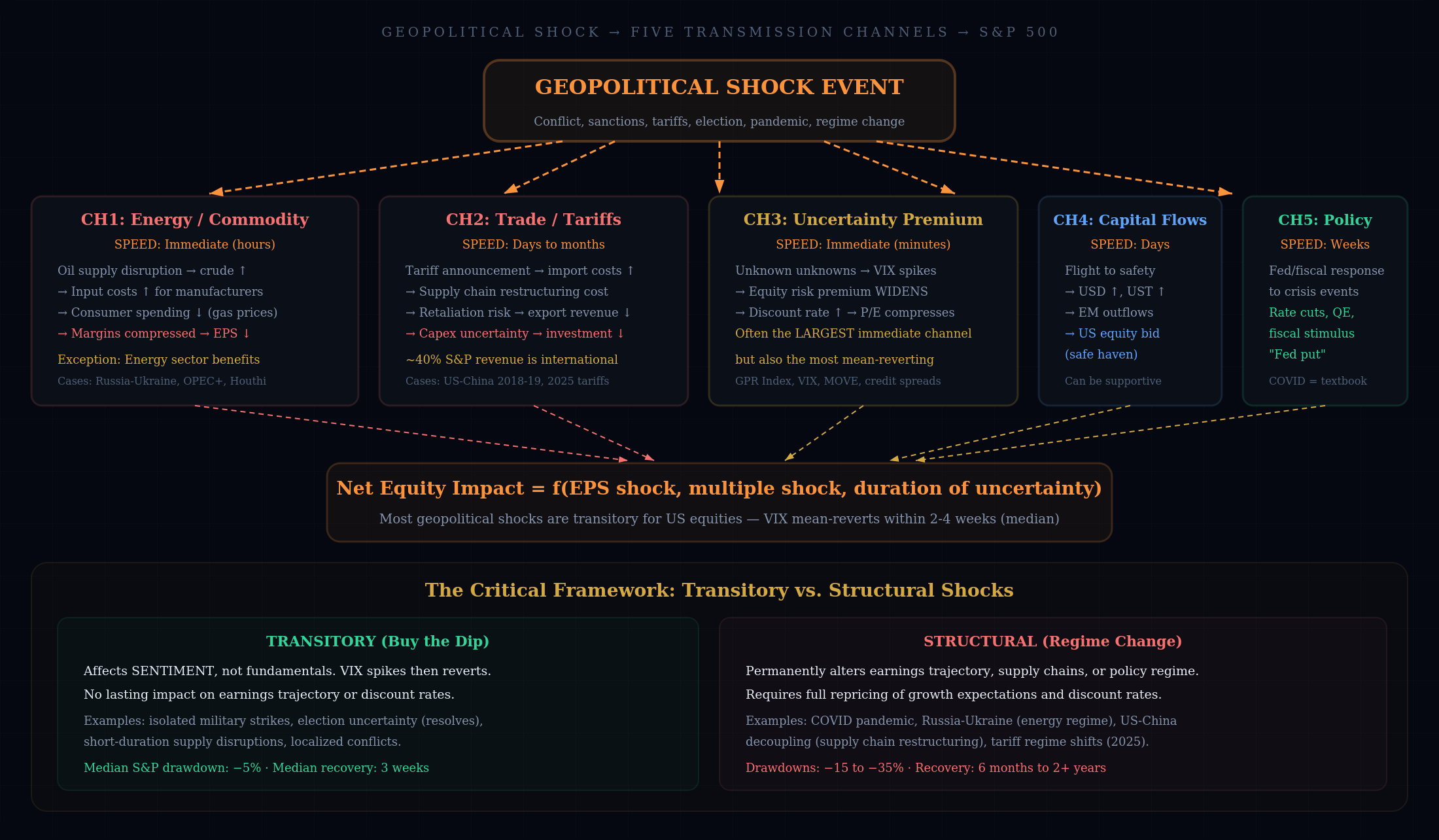
The 5 channels are: energy and commodity supply disruption (immediate, affects margins and input costs), trade policy and tariff escalation (days to months, affects revenue and supply chain costs), uncertainty premium (immediate, affects the VIX and equity risk premium), capital flight to safety (can paradoxically support US equities), and policy response (the “Fed put” that often follows crises).
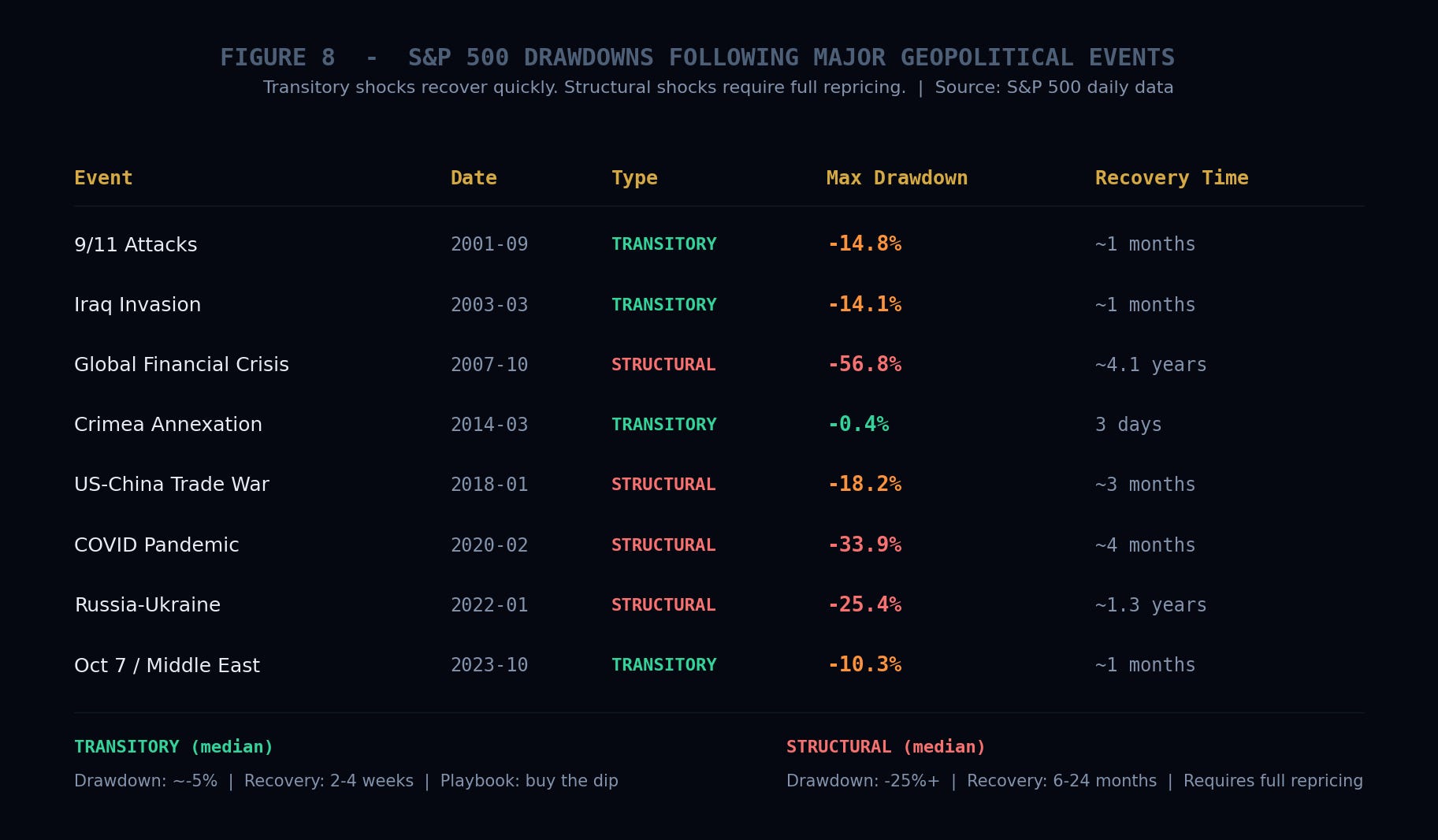
The critical analytical question with every geopolitical shock is: is this transitory or structural?
Transitory shocks affect sentiment but not fundamentals. The VIX spikes, the market sells off 5 to 15%, and within a few weeks prices are back to where they started. Structural shocks permanently alter the earnings trajectory, supply chain architecture, or policy regime, requiring a full repricing.
I have lower conviction in my ability to predict geopolitical events (obviously), but I have high conviction in the framework for assessing their transmission once they occur. The key question is always: does this change the earnings (EPS) trajectory, or does it only change sentiment (P/E Multiple) temporarily?
How these forces interact: the regime framework
The real analytical value of this 5 factor framework isn’t in understanding each force independently. It’s in understanding how they interact.
When multiple forces push in the same direction, the moves are large and persistent. The 2020 to early 2022 rally saw all 5 forces aligned bullishly: massive QE, enormous fiscal stimulus, pandemic driven positioning washout, no geopolitical headwinds, and an earnings recovery from the COVID trough. Everything pushed the same way. The S&P roughly doubled.
The 2022 bear market was the reverse: QT launched, fiscal tightened, inflation was eroding margins, positioning was crowded long, and the Russia/Ukraine shock hit energy costs. Most of the forces flipped bearish simultaneously, producing a 25% decline.
The most interesting (and profitable) regimes are when the forces conflict. The 2023 to 2024 period is the best recent example: QT was running (bearish for liquidity), but the RRP drain was more than offsetting it (bullish for liquidity). Fiscal deficits were enormous but funded primarily through bills not coupons (neutral to bullish for term premium). Earnings growth was moderate but positive. Positioning was light and progressively loading up.
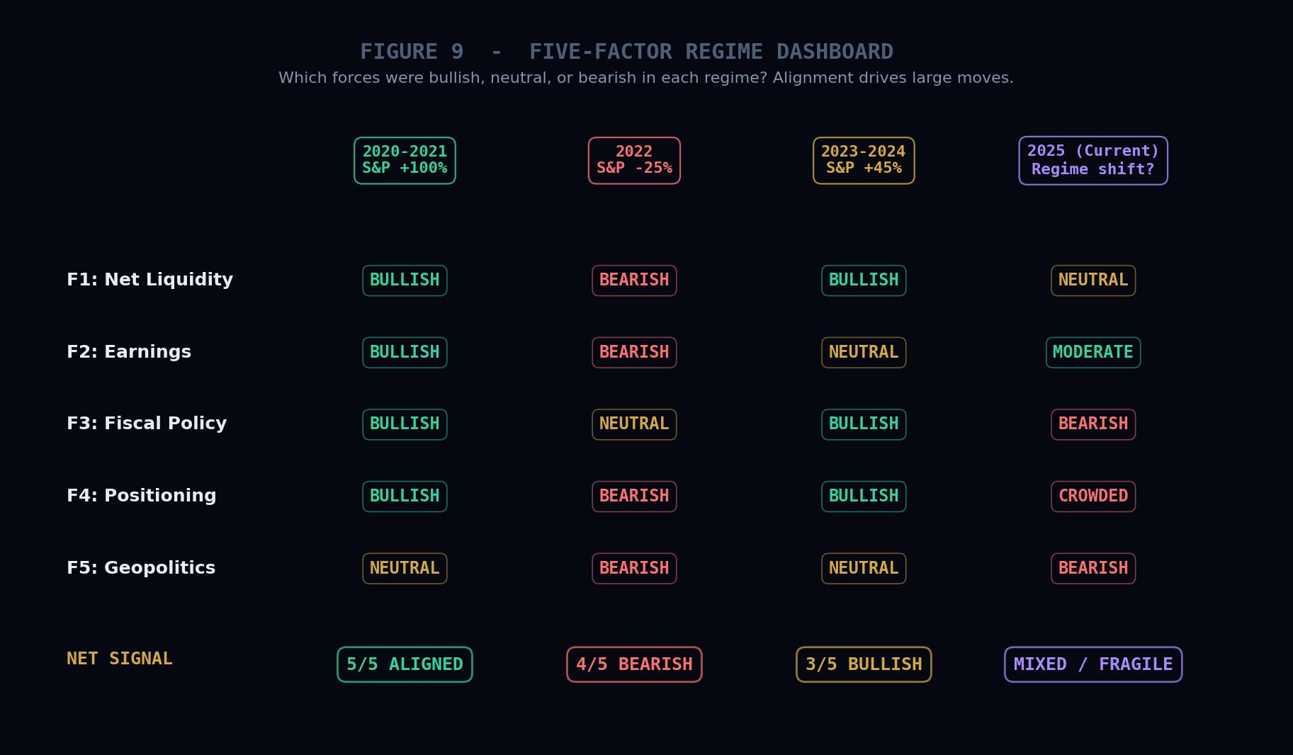
The question I’m always asking myself is: which force is dominant right now, and is the market correctly pricing it?
Time horizon matters: which force dominates when?
Not all forces are equal at all times. One of the most important calibrations in this framework is matching the right force to the right time horizon:
1 to 6 months: Net liquidity and positioning dominate. Over short windows, the P/E multiple is the primary driver of returns, and the multiple is set by liquidity conditions and how the market is positioned.
1 to 5 years: Earnings growth dominates. The multiple mean reverts over time. What compounds is EPS growth, driven by revenue cycles, margin dynamics, and share buybacks.
10 plus years: Valuation at entry dominates. Both the multiple and the earnings cycle mean revert. The Shiller CAPE at your purchase date has historically explained roughly 80% of the variance in subsequent 10 year annualized returns.
Always Remember: the future investment returns generated from an asset are directly related to the price one pays for said asset, particularly over longer time horizons.
The practitioner’s monitoring toolkit
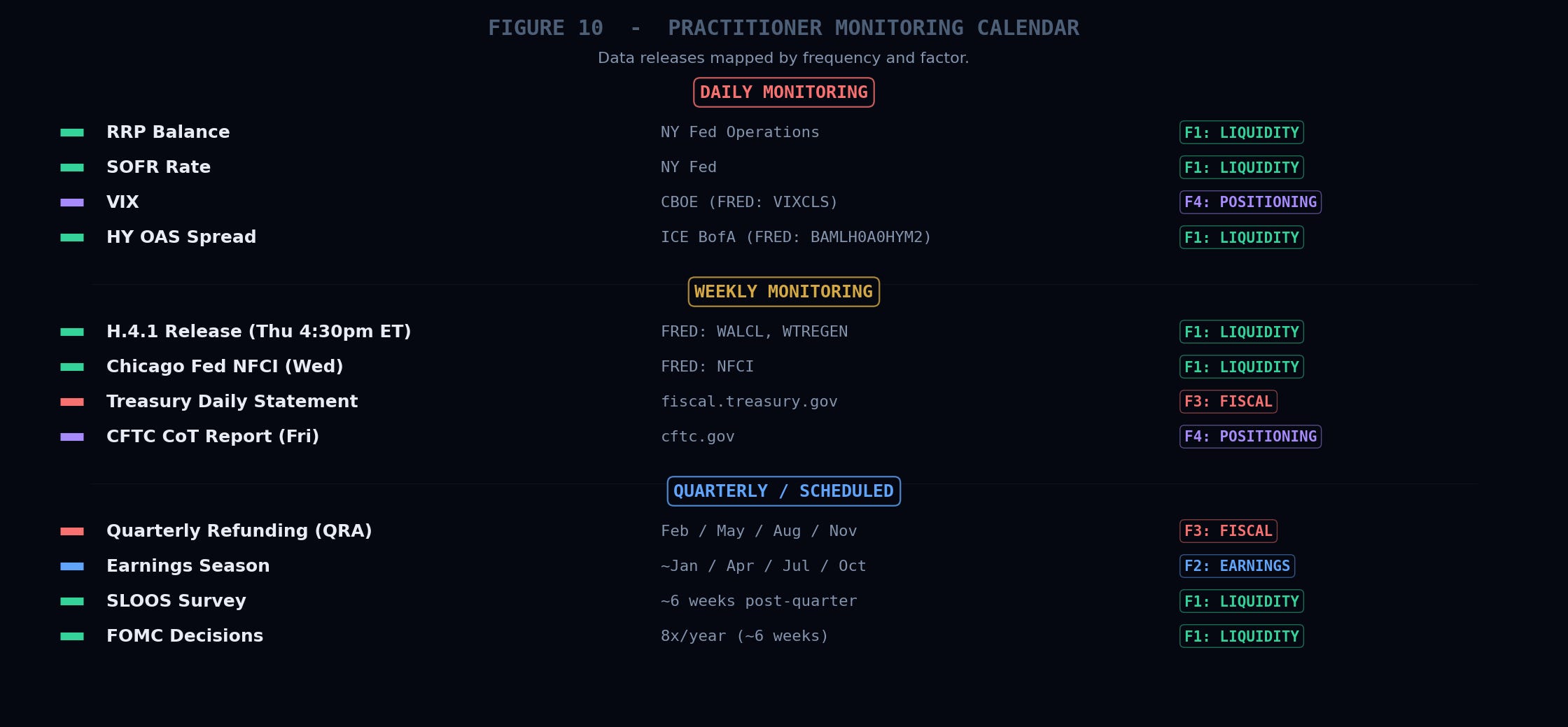
Knowing the framework is one thing. Monitoring it in real time is another. Here’s what I track and when:
Weekly (Thursday, after the H.4.1 release at 4:30pm ET):
Compute net liquidity from FRED: WALCL minus WTREGEN minus RRPONTTLD.
Compare the weekly change to the trailing four week average.
Flag any single week move larger than $100 billion and investigate the source.
Daily:
RRP balance from the NY Fed’s daily operations page.
SOFR rate relative to IORB (if the spread exceeds +10 basis points, funding stress may be emerging).
VIX level and credit spreads (HY OAS from FRED series BAMLH0A0HYM2).
Quarterly:
Earnings season: track revision breadth.
Treasury’s Quarterly Refunding Announcement (February, May, August, November): the bill vs coupon issuance mix is the single most important signal for the fiscal to liquidity channel.
Senior Loan Officer Opinion Survey (SLOOS)
As Needed:
CTA positioning estimates from Goldman Sachs or JPMorgan.
Dealer gamma exposure estimates from SpotGamma.
Geopolitical risk premium proxies (GPR Index from Caldara and Iacoviello).
The monitoring calendar below maps every data release by frequency and by which of the 5 forces it corresponds to.
Conclusion:
Understanding what moves equity prices requires holding 5 forces in your head simultaneously. That sounds like a lot, but the framework simplifies to a single decomposition: Price = EPS x Multiple. The fundamental forces (earnings, fiscal stimulus) drive EPS. The financial plumbing forces (liquidity, positioning) drive the multiple. Geopolitics can hit either one.
The regime you’re in (which forces are dominant, which are aligned, which are conflicting) changes over time. The analyst’s job is to identify the regime correctly and monitor for shifts. The biggest analytical errors I see come from investors who are anchored to one force while a different force has taken the wheel.
I hope this framework is useful to you. It’s taken me quite awhile to develop and it continues to evolve. My suggestion: start by monitoring net liquidity on Thursdays after the H.4.1 release. That single weekly data point will change the way you think about the market.
— Brant
If you found this analysis useful, please like, subscribe, and share. Your readership is much appreciated.
Disclaimer: The content provided on the Capital Notes newsletter is for general information purposes only. No information, materials, services, and other content provided in this post constitute solicitation, recommendation, endorsement or any financial, investment, or other advice. Seek independent professional consultation in the form of legal, financial, and fiscal advice before making any investment decision. Always perform your own due diligence.